9 Succession Lab

9.1 Introduction to the lab

Several habitat types can be discerned during a walk through BFL, each representing the integration of biotic and environmental factors with disturbance history. Here we look at species composition and age structure of trees that characterize some of these habitats.

The relative abundance of different size classes of various tree species in a forest can provide clues about the history and future status of those species in that forest. For example, even if a tree species is abundant, yet represented only by large, older individuals, it is likely that the requirements for seed production or seedling establishment in the area have not been present in recent times. In order to predict the future status of that tree species in a given area we would need to find out about its requirements for regeneration and determine the likelihood that such conditions will be repeated during specified time periods. For example, for a species that requires a fire to germinate and establish, we would need to predict when fires are likely.

In contrast, a tree species represented by a large population of saplings (presumed from their size) must have recently enjoyed favorable conditions for reproduction and establishment. Will such a species therefore dominate a future forest on the site? Possibly, but this may be difficult to answer since factors like disease, herbivory, fire, and/or shading by faster growing competitors may affect the survivorship of this cohort over time. Studying the size or age structure of a population helps ecologists make such projections. (Note that we generally assume that big trees are older than smaller individuals of the same species, but keep in mind that individuals of the same size may differ in age and vice versa. Local variation in microclimate edaphic factors (having to do with the soil) and light environment may result in rather different trajectories of growth for identical seedlings germinating the same year.)

The goal of this project is to acquaint you with some of the kinds of data ecologists collect in attempting to answer questions about population trends. This exercise will also expose you to the always-messy issue of how to collect field data, and to give you insight and experience in statistical analyses appropriate for testing hypotheses about differences between species within different habitats in the age/size structure of trees. We will observe and quantify the distribution, abundance and size structure of dominant tree species at BFL. However, in collecting data to describe densities and size structures of these species at BFL, we are in position to test whether species have responded differently to major variations in the habitat at BFL. Once we have collected data on the trees with respect to variations in habitat at BFL, the patterns observed may stimulate additional questions and hypotheses.

9.2 Materials and Methods

9.2.1 BFL habitat regions

To collect data we will establish transects in three areas of interest: the lower river terrace, the old pastures (experimental plots) and the quarry zone (see figure 9.1 for a map).

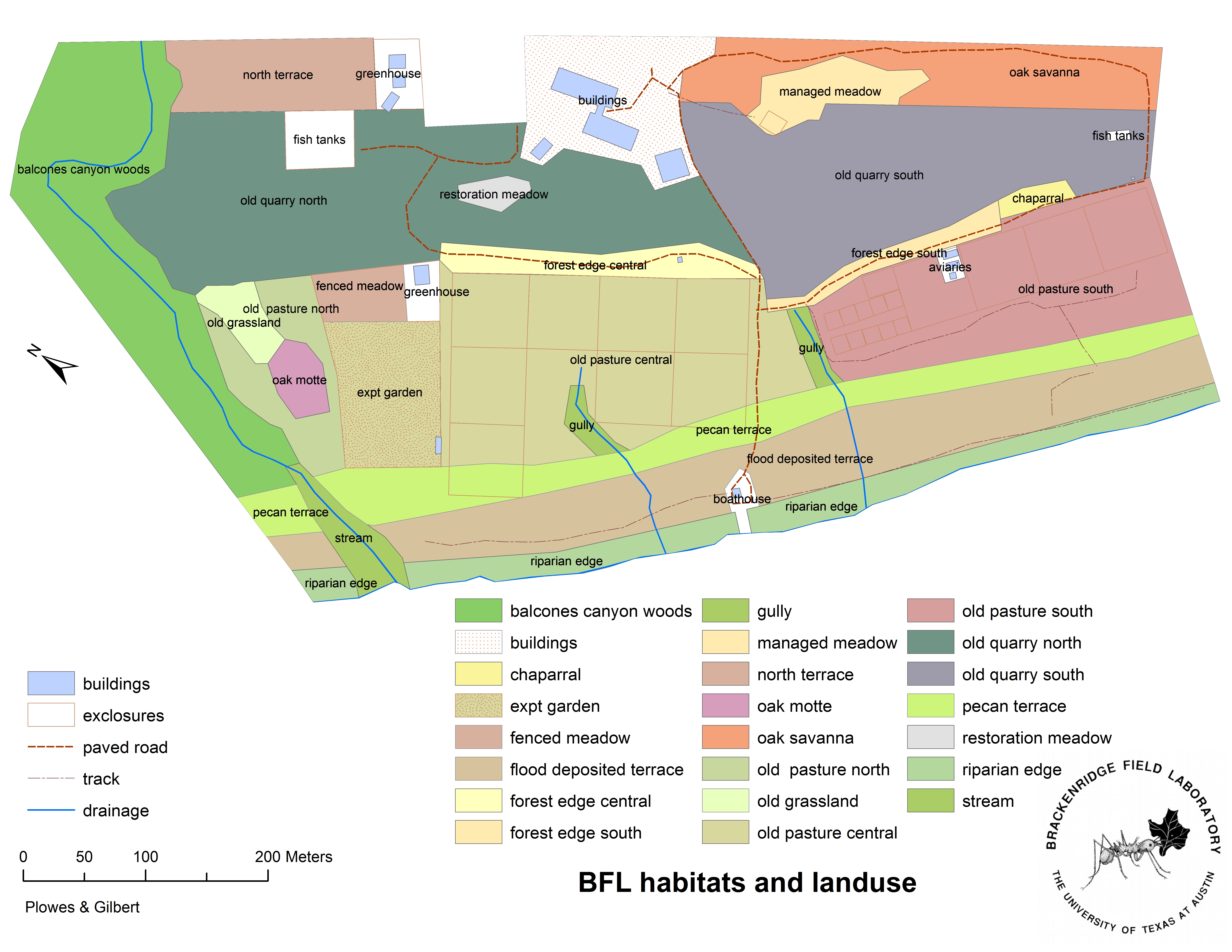
Habitat map of BFL; for the purposes of this lab, the river terrace corresponds to the pecan terrace and flood deposited terrace (near the bottom), the old pasture is the central area, and the old quarry is near the top.

Figure 9.1: Habitat map of BFL; for the purposes of this lab, the river terrace corresponds to the pecan terrace and flood deposited terrace (near the bottom), the old pasture is the central area, and the old quarry is near the top.

9.2.2 Data Collection

Given the brief time allowed by the class period, we don’t count absolute numbers, but instead use sampling techniques for describing tree populations and habitats.

We will use the Point-Quarter Technique to collect data (Cox p. 66). The beauty of this method is that it allows us to quickly estimate the density of selected species in the community while gathering information on their relative abundances.

Each team will perform a survey in each of 3 apparently distinctive habitats.

9.2.2.1 Point-quarter for quarry and river terrace habitats

Sample Point selection:

Starting with an existing transect marker in the zone your team is assigned, flip a coin (or use a random number generator) to determine direction (left or right) that you will take perpendicular to the trail.
Use a random number generator app to pick a number between 10 and 39 (alternatively, have one team member think of a number between 1 and 3 and another between 0 and 9). Your first point will this many meters from the trail in the predetermined direction.
Repeat this process at the next transect tag, but in the opposite direction.
Repeat it a third time for a total of 3 sample points in the habitat.

Note: Areas recently cleared or plowed should be excluded.

Each sample point is to be temporarily marked with a flag (do not leave any flags behind!!). The 3 sample points along each transect represent the center of four quadrants with sides along and perpendicular to the transect line.

In each quadrant, you will determine the nearest canopy tree and sapling to the center point. Canopy trees are defined as having a crown that is exposed directly to sunlight and forms part of the overhead canopy. Saplings occur under the crown of canopy and are assumed to be potential canopy replacements when the canopy tree dies.

Data to collect from each point:

Location (with UTM)
Species of nearest canopy trees & saplings
Distance of these trees from the center point
Diameter at breast height (dbh) of canopy trees
Note signs of drought stress (leaves are wilted or dead/brown)

9.2.2.2 Point quarter for old pasture habitat (pond enclosures)

Sample Point selection:

Because there are edge effects around enclosure walls and there is a pond in the center, we are primarily concerned with the forest that came into the sapce between the path around the wall and the pond dam, replacing the pasture that Dr. Gilbert saw as a student in 1964.

From the pond in the center of the acre, select three points along the radius of the inner circle. For each point, enter the forest surrounding the pond and go about halfway to the wall. Complete your point-quarter surveys from there.

9.3 Analysis to perform

You should provide data and analyses to address the following questions:

What are the qualitative trends and characteristics of each habitat?
How does the total density of canopy trees differ between habitats?
Does relative abundance of each species differ between canopy and sapling trees? How consistent is this among habitats?

Remember: describe what analyses you did in the method section, present what your found in the results section, and talk about what it means in the discussion.

9.3.1 Canopy tree density

You can use the point-quarter method to estimate tree density at each site with a bit of math. Let \(x_i\) be the distance from your point to a sampled canopy tree. If you sampled 4 trees at a point, then the density in trees per square meters would be \(\frac{4}{x_1^2 + x_2^2 + x_3^2 + x_4^2}\). More generally, the density is \(1 / \text{mean}(x^2)\).

Calculate density for each sample point, and convert it to hectares (multiply by \(10,000 \text{ m}^2/\text{ha}\)). How do densities compare between habitat types? Create a figure and compare the averages. Note that you won’t be able to claim that one group is different unless you use statistical tests, such as a one-way ANOVA (this is optional).

9.3.2 Species by habitat and life stage

For each habitat, you will want to calculate the relative abundance of each tree species for canopy and sapling trees (i.e., number of Canopy species x in habitat y divided by total number of observed Canopy trees in y). Visualize the result for each habitat (a three-panel frequency plot would be the best way to go, with categories ordered by canopy abundance).

To test if the relative proportions in canopy and saplings are equivalent, you should construct contingency tables for each habitat (See Table 9.1 for an example). Restrict each table to the five most common species in each habitat. Contingency tables can be constructed with pivot tables in Excel or the table() function in R. Use chi-square tests to see if the proportions of species are different between canopy and saplings for each habitat.

Table 9.1: Abundance of most common canopy and sapling trees in the BFL old pasture habitat, Fall 2018.
	Carya illinoiensis	Celtis spp.	Juniperus spp.	Quercus buckleyi	Quercus fusiformis	Ulmus crassifolia
Canopy	7	2	17	3	2	9
Sapling	0	6	7	3	6	11

9.4 Discussion

Some suggestions for discussion topics:

How could differences in sapling/canopy relative abundances inform possible successional trends? Based on your results, what would you predict about future dominant species in the habitats?
Did you observe anything else about the ecology or natural history of these areas that may help account for your results (e.g., drought stress, dead trees, invasive species, disease, etc)?
What may be driving the differences in the habitat types? Considering the history of BFL may be helpful in explaining some of this.
Develop a likely scenario for the past and future decades of tree population dynamics in the woodlands of BFL.
How has drought and oak wilt affected the tree community at BFL? How might a scenario for succession based on currently healthy trees be changed if we include the information on stressed/dead trees?
How could this line of research be expanded upon in future work?

9.5 General Comments (Post-Review)

These were some general comments I had on a previous year’s reports; I’d recommend reading them, since they’re common mistakes that it would be good to avoid.

9.5.1 Figures

Review the guidelines in the Figures chapter. Specifically:

Don’t use figure titles; anything that could go there should be in the caption instead.
Use colors that will work in black and white,
Number figures in the order they’re cited in the main text; they should also be arranged in this order (e.g., figure 2 shouldn’t be placed before figure 1).
If the figure contains new data (which all of these should), it should be cited in the results.
Figure numbers shouldn’t have decimals in them (e.g., no Figures 1.1, 2.3, etc). If you have a multi-panel figure, refer to specific panels as Figure 1a, 1b, etc.
If you have a multi-panel figure, there should be a single caption that explains what each of the panels are.
Don’t use bar plots for group means; boxplots or violin plots are usually better. This is a very inefficient way to present 3 data points, and it provides no information about the data’s variability. Boxplots or violin plots are better options. (Note that bar plots are still fine for counts or proportions).
No gridlines (see below)

To remove gridlines in excel, just click on them and delete them. Base plots in R (with the plot() function) shouldn’t have them by default. To remove them with ggplot2 figures, put this near the top of the code:

install.packages("cowplot") # if you don't have this installed; run once
library(cowplot)
theme_set(theme_cowplot()) # this makes your ggplots look nicer until you restart R
# ggplot commands here

9.5.2 Write this like you’re trying to publish it

You should write these reports as if you were writing a manuscript for a journal. Pretend it’s not a class paper; don’t say “For this lab, our assignment was…” or “the other students…” Write like it’s a research project; you came up with the hypotheses and methods and the other students in the class are your collaborators.

When describing the data collection, you need to describe how all of this year’s data was collected, for all groups. Instead of saying “we sampled three points in per habitat,” say “five groups each sampled three points per habitat.” As part of this, don’t talk about combining your group’s data with the rest.

Finally, you need to have a real title.

9.5.3 Describe the habitats

Since the different habitat types are an important part of this paper, you should describe them in a reasonable amount of detail; this could go in the intro or methods section, depending on how you wrote it.

9.5.4 The Analysis

Formally, the chi-squared test evaluates whether the rows and columns of a contingency table are independent of each other. In the context of this project, that’s equivalent to testing whether the Canopy:Sapling ratio was equal for each species OR if the prevalence of each species was the same for canopy and sapling trees.

Several people misinterpreted the analysis as examining if there were more canopy or sapling trees. This wouldn’t work, because the chi-square test cannot tell you anything about the actual number of trees and because the way you collected the data (a fixed number of trees per point) was not set up to answer this question.

The Chi-square analysis was often described incorrectly in the methods; an unfamiliar reader would not know what you were testing. When you’re describing the test, you don’t necessarily need to state the null/alternative hypotheses, but you need to make it clear what question you’re answering with it.

It’s also worth remembering that the data we collect is generally not incredibly high precision. Our measurements generally don’t have the ability to distinguish between a mean density of 437.11 and 437.14; depending on the sample size, we may not even be able to distinguish between 437 and 442. Being overly precise doesn’t help. If your p-values are less than 0.0001, just report “p < 0.0001.”

9.5.5 Keeping things in the right sections

Many people restated the methods used for their statistical analyses in the results. For example:

“I ran chi-squared tests, and they showed significant differences in the old quarry (chi-square = …, df = …, p = …), the old pasture (…) and the river terrace (…).”

Don’t do this; instead, only provide the result. A better re-work of the above sentence would be:

“Species composition was significantly different between canopy and sapling trees in the old quarry (…), the old pasture (…), and the river terrace (…).”

Don’t put anything in the intro or methods that is actually a result. Many people listed the most common species found in each habitat in their “study area” sections. Since this was a major part of this lab, listing the dominant species should be accompanied by a citation to show evidence that this is already known. In general, if you find yourself saying that the most common species “were” something, then it sounds like you are talking about your own observations; if you say that they “are” or “have been” something, then it sounds like you’re talking about more general patterns.

9.5.6 Basic style and format rules

Don’t capitalize things that don’t need capitalization (e.g., the point-quarter technique).
Most acronyms should be defined before their first use (though there are a few exceptions, like ANOVA).
Don’t say (p-value = x), say (p = x).
If a paper has more than two authors, cite it as “(Smith et al., 2009),” not “(Smith, Johnson, Franks, and Brown, 2009).

9.5.7 Other Comments

The “fisher test” is properly called Fisher’s exact test (with “Fisher” capitalized).
If you used a stats program for a bunch of different things (as you usually do w/ R or Excel), mention it at the end of the section, not the beginning.
RStudio is an interface for doing analysis with R; if you used it, you should say you did your analysis in R.
Make sure to explain that sample points were selected differently in pond/old pasture than in other habitats.
In the discussion, if you are listing several possible interpretations of your results, it’s a good idea to put the most interesting one(s) ahead of the “this is all random noise” option.