15 Homework: Heterogeneity
15.1 Required Reading
This homework will prepare you to analyze the data from the Heterogeneity lab. You should read over that the material to properly understand the data you’ll be working with here. I will assume that you are familiar with the material used in the Succession homework (which references Chapters 4, 5, and 6, and Sections 7.1 and 7.2). In addition, you should read Section 7.3.
15.2 Objectives (and what’s due)
What are the relationships between canopy, shrub, and ground cover?
- Submit: Colored contingency tables for Canopy x Shrub, Canopy x Ground, Shrub X Ground, and interactions.
- Submit: Chi-squared or Fisher’s Exact tests that correspond to these contingency tables
How do the relative abundances of Canopy, Shrub, and Ground cover compare with historical observations?
- Submit: Colored contingency tables for current vs historical levels of Canopy, SHrub, and Ground cover.
- Submit: Chi-squared or Fisher’s Exact tests that correspond to these contingency tables
You’ll also be doing to other things that aren’t specifically hypothesis or question driven, but should be presented in the results.
Calibrating your subjective estimates of canopy estimates with the Gap Light Analyzer calculations. This in particular isn’t a biological hypothesis, but comparing different methods for addressing the same question is a common feature of biological research.
- Submit: A regression of subjective canopy score vs. percent canopy opennesss, with an associated figure.
15.3 Getting started
You should download two datasets from Canvas and put them in your data folder:
- F20_heterogeneity_data.csv: The “current” dataset.
- historical_data_Fall_03_to_19.csv: contains data from most fall semesters since 2003.
Begin your script with the following:
Save the R file as R/heterogeneity_homework.R.
15.4 The data
The columns of these data frames that are relevant are:
- Tag: transect tag number
- Ground, Shrub, Canopy: subjective scores for these three layers, ranging from 0 (empty) to 3 (fully closed).
- Percent_Cnpy_Open (current) or percent_ca (historical): Percent canopy openness, as determined by Gap Light Analyzer; higher values indicate a more open sky.
- Season and Year (only in historical); when the data were collected.
15.5 Relationships between Cover Levels
Using the current data, create contingency tables for each pairwise combination of Canopy, Shrub, and Ground (three tables total); for each of these, run chi-squared tests (or Fisher’s tests if necessary). Instead of including the contingency table directly, we’re going to create figures that show colored heat maps.
your_contingency_table |> # replace with your contingency table name
as_tibble() |> # Convert to a data frame
ggplot() +
aes(x = , y = ) + # Finish these
geom_tile(aes(fill = n)) + # Makes colored squares based on count
scale_fill_viridis_c() + # Nice color scale
coord_fixed() + # keeps x & y dimensions equal
# Add text to the squares
geom_label(aes(label = round(n, 3)), # Include the count as a label; the rounding is there in case you want to switch it to a proportion
label.size = 0, # Keep this as is
# Feel free to adjust these details
# to get an image you like
color = "white", # Text color
fill = "#00000010", # Slight background around text to make it more legible
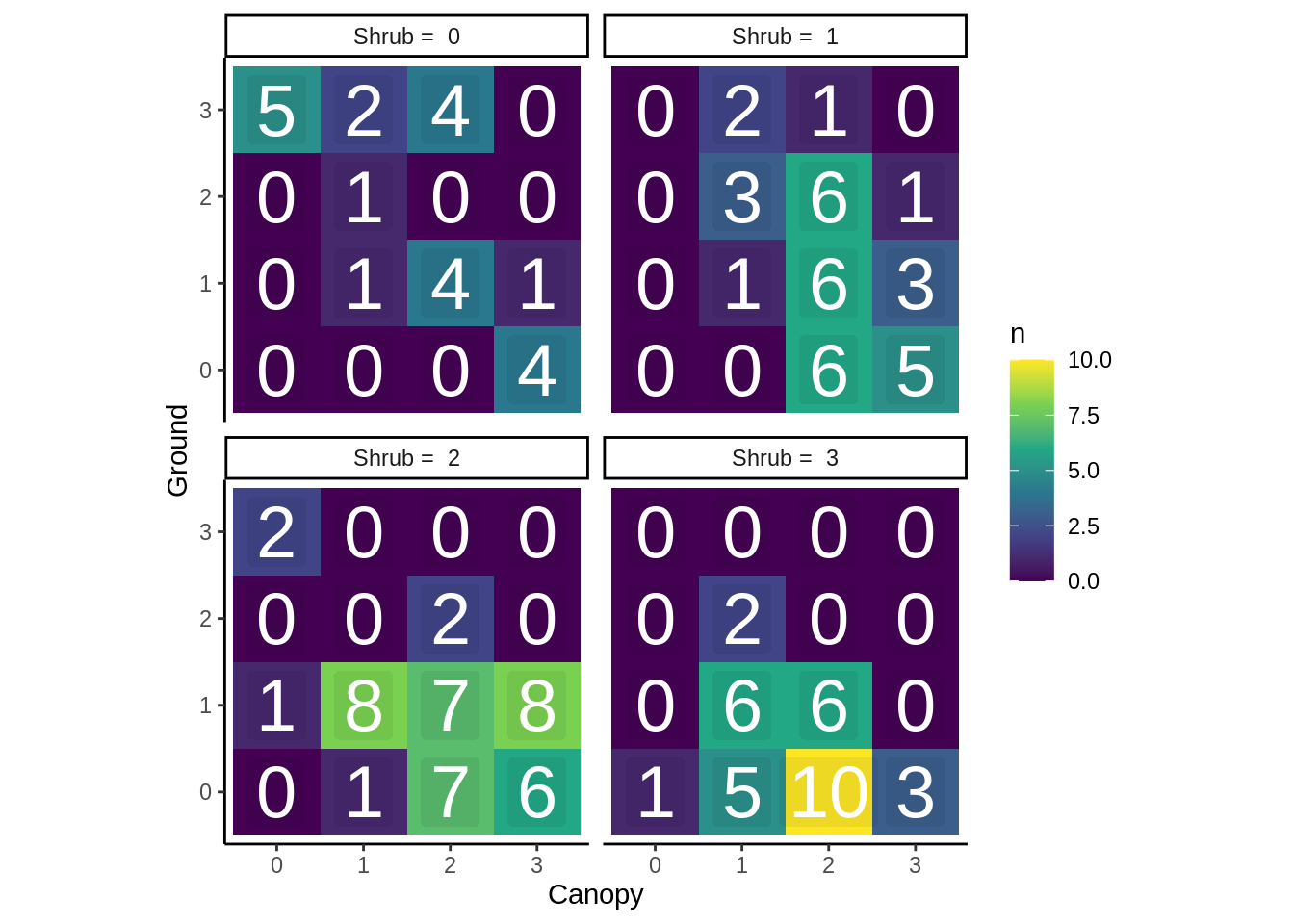
size = 10) # text size; To look at the interaction of all three levels, create four data sets for each different shrub level using the filter() function and run separate Chi-squared / Fisher’s exact tests.
To visualize the table, you’ll need to make a 3-dimensional contingency table and manipulate it:
contingency_3d <- current_data |>
  select(Canopy, Shrub, Ground) |>
  table() |>
  as_tibble() |>
  mutate(Shrub = paste("Shrub = ", Shrub)) # Modify shrub to include the label; this will help with faceting
Then use this with the figure-making code, but use facet_wrap() (Section 5.4) to make separate panels for each shrub level.
Your final figure for this should look like this:
15.6 Relationship Between Current and Historical Cover Levels
You’ll need to make a dataset that contains the current data and the semester of interest (which is Fall 2004).
First, filter historical_data_full so that it only includes Fall 2004’s data (save as historical_data_F04).
Then, you’ll want to modify the current_data so that it has columns for the Semester and Year (Fall 2020) before binding it to the 2004 data:
historical_comparison_data <- current_data |>
  mutate(   ) |>  # Fill this in; new columns should match the columns in historical_data_full
  bind_rows(historical_data_F04) # Combine w/ F04 data
From here, you’ll need to make 3 more contingency tables (Year vs. each of the cover levels), run the appropriate tests on them, and visualize them.
15.7 Calibrating Subjective Scores with Gap Light Analyzer
The cover levels here are subjectively determined; it’s probably a good idea to see how well the subjective scores match with a more objective measure.
We’ll do this with a linear regression (Section 7.3).
To see how well subjective scores predict the GLA percent canopy openness, run a regression with Canopy as the predictor (X) and Percent_Cnpy_Open as the response (Y).
When reporting these results, focus on the \(R^2\) statistic, as it indicates the amount of variation in canopy openness is explained by the subjective scores.
Create a figure of the regression with both a regression line and individual data points (See 5.3.3 for examples).
For the data points, use geom_jitter(height = 0, width = 0.15) instead of geom_point(), so that all of the points aren’t lined up with each other.