14 Homework: Succession
14.1 Required Reading
This homework will prepare you to analyze the data from the succession lab. You should read over that the material to properly understand the data you’ll be working with here. Information on the data-analysis techniques you’ll need to use can be found in Chapters 4, 5, and 6, as well as Sections 7.1 and 7.2.
Please attempt this to the best of your ability. Once you’ve read the above chapters, I will be happy to meet with you (individually or in groups) to provide guidance and support on this material.
14.2 Objectives
The analysis for this lab should answer:
- Is there a difference in the relative abundances of species between canopy and sapling trees in each habitat?
- Does canopy density differ among habitats?
14.2.1 What’s due?
- A 3-panel figure that shows the relative abundance of canopy vs. sapling trees in each of the 3 habitats. You can create each panel separately, as long as they’re presented together with a single caption.
- For each habitat, a contingency table that shows the abundance of canopy and sapling trees for the 5 most abundant species in that habitat.
- A chi-squared test or Fisher’s exact test for each contingency table, along with 1 sentence reporting the results (e.g., significant differences).
- A figure showing the distribution of canopy densities among the three habitats. Should include a caption.
These should be submitted as a Word document or PDF. The figures and tables you create should follow the guides in Chapter 3.
14.3 Getting started
As this is the first stats homework, let’s make sure you’re using RStudio correctly.
14.3.1 Make sure your software is up-to-date
Check R Version: Open RStudio. In the Console, your R version should be listed. If it is less that 4.0, you need to re-install R. Download R here.
Check RStudio Version: Go to Help -> About RStudio. If the version listed is lower than 1.4.1717-3, then you need to re-install it. Note that very recent versions are numbered with a date (e.g., v. 2021.9.1.372); these are good. Dowload RStudio Desktop here.
Check package versions: In the console, run library(tidyverse).
If this fails, run install.packages("tidyverse"), then start this over again.
Tidyverse is a collection of packages that are designed to work well together.
You should see the header “Attaching packages”, followed by a list of package names and version numbers.
Make sure that the following packages are at least this high:
ggplot2: 3.3.3tibble: 3.1.0tidyr: 1.1.3readr: 2.0.0purrr: 0.3.4dplyr: 1.0.5stringr: 1.4.0forcats: 0.5.1
You should also click the packages tab in one of the RStudio panels and verify that you have the following:
-cowplot -vegan -ggforce
If any of these are missing or out of date, use install.packages(c("package1", "package2", "etc")) to get them.
14.3.2 Create the RStudio Project
In the upper-right corner of the RStudio window, there should be a box that says Project: (None). Click this, then on the drop-down menu select New Project...
If you already have a folder on your computer for Bio 373L, select Existing Directory, then hit Browse and navigate to that folder. Otherwise, select New Directory -> New Project, and name the directory “Field Ecology” or “Bio 373L” or whatever; place it as a subdirectory wherever you normally keep your class files. Click Create Project.
RStudio will refresh, and it should now say BIO 373L or whatever you named the project in the upper right corner. Whenever you open RStudio for this class, make sure the project name is there. If it isn’t, click that box and you should be able to select the project from the drop-down menu.
Click on the Files tab (in one of the RStudio panels). This will give you a list of files & folders that are part of the RStudio project. From here, use the New Folder button to create the following subdirectories:
data: for raw data filesR: for saving script filesoutput: for saving the results of your analysesfigures: for saving graphs
Organizing your project like this is a good way to keep your files tidy and easy to find.
14.3.3 Create an R script.
Create a new R script with Ctrl + Shift + N or File -> New File -> R Script. This will open up the script panel.
Start your script with this code:
# Succession Lab Analysis Homework

## Setup ####
# Load Required Packages
library(tidyverse)
library(cowplot)
Put your cursor on each line and hit Ctrl + Enter (or Cmd + Return on a Mac).
This will send that line to the console and run it.
Entering your commands in a script makes it a lot easier to see what you’ve done, repeat it, or modify it.
You should only enter code in the console if you don’t want a record of it (which should be an unusual circumstance).
Save your script as R/hw_succession.R
14.4 The Data
For the homework, we’ll use a dataset in Fall of 2019.
14.4.1 Download and import the data
Download succession_long_F19.csv and save it in the data folder.
To read and view the data, add the following lines to your script and run them:
succession_data <- read_csv("data/succession_long_F19.csv")
View(succession_data)
Note that I used read_csv(), not read.csv().
Always use the version with the underscore; it’s part of the readr package (which is part of tidyverse) and is generally faster and more consistent than read.csv().
RStudio also has a data import tool.
Do not use it.
You should import your data with code so that you can go back later and see exactly what you’ve done.
14.4.2 Data
Your data should look something like this:
| Habitat | point_number | Team | Quadrant | Location | Location_type | Location_angle | Tree_type | Distance | DBH | Drought_stress | Species | N_dead |
|---|---|---|---|---|---|---|---|---|---|---|---|---|
| P | 1 | A | a | Pond G | Pond | 11 | Canopy | 3.30 | 14 | FALSE | Carya illinoiensis (Pecan) | 0 |
| P | 1 | A | b | Pond G | Pond | 11 | Canopy | 2.90 | 27 | FALSE | Carya illinoiensis (Pecan) | 0 |
| P | 1 | A | c | Pond G | Pond | 11 | Canopy | 1.60 | 21 | FALSE | Carya illinoiensis (Pecan) | 0 |
| P | 1 | A | d | Pond G | Pond | 11 | Canopy | 2.90 | 32 | FALSE | Carya illinoiensis (Pecan) | 1 |
| P | 1 | A | b | Pond G | Pond | 11 | Sapling | 1.30 | NA | NA | Fraxinus texana (Texas ash) | 0 |
| P | 1 | A | c | Pond G | Pond | 11 | Sapling | 2.60 | NA | NA | Carya illinoiensis (Pecan) | 0 |
| P | 1 | A | d | Pond G | Pond | 11 | Sapling | 4.60 | NA | NA | Broussenetia papyrifera (Paper mulberry) | 0 |
| P | 2 | A | a | Pond G | Pond | 3 | Canopy | 3.90 | 21 | FALSE | Juniperus ashei (Ashe’s Juniper) | 0 |
| P | 2 | A | b | Pond G | Pond | 3 | Canopy | 0.98 | 19 | FALSE | Carya illinoiensis (Pecan) | 1 |
| P | 2 | A | c | Pond G | Pond | 3 | Canopy | 1.95 | 30 | FALSE | Carya illinoiensis (Pecan) | 0 |
This data is in a tidy format: each row is an observation (a single recorded tree), each column is a separate variable. These are the columns that are relevant to the analysis:
- Habitat: Indicates if samples were taken from the Old Quarry (Q), the Old Pasture (P) or the River Terrace (R).
- point_number: Each point in a point-quarter sample has multiple observations (8 for the old quarry & river terrace, with 4 quarters of canopy and sapling trees) or 4 for the old pasture (2 quarters each). This column identifies each separate point.
- Tree_type: Indicates if the row records a canopy or sapling tree.
- Distance: Distance in meters from the point to the tree (only for canopy trees).
- Species: Species of the tree.
The remaining columns (Team, Quadrant, Location, Location_type, Location_angle, DBI, Drought_stress, N_dead) are not relevant to this analysis and can be ignored.
Lets trim this data by removing the unnecessary columns.
Use a select() function to make a copy of the data that doesn’t have the unnecessary columns. Save the resulting data frame as succession_data_thin.
(See section 6.4; section 6.1 is also helpful).
14.5 Comparing the relative abundance of canopy and sapling trees in each habitat
You’ll need to filter() your data (see 6.3) so that it only contains a single habitat when doing these comparisons.
Let’s start with the old quarry; once you get everything working, you should copy and modify the code to work for the other two habitats.
You should also read up on the pipe ( |> ), as it is important for making sequences of steps (6.1).
## Relative Abundance - Q ####
data_Q <- succession_data_thin |> filter(Habitat == "Q")
Comment lines ending with #### are a good way to organize different sections of your code. RStudio will allow you to collapse the code underneath it (until the next section), so you can navigate your document more easily.
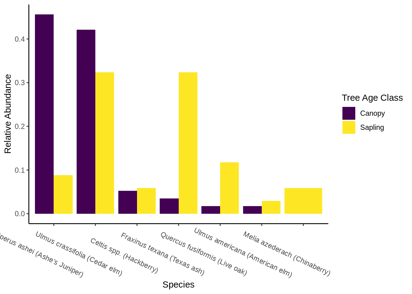
14.5.1 Create a barplot comparing canopy & sapling abundances
For each habitat, you’ll need to create a bar plot comparing the relative abundances of canopy and sapling species. It should look something like this:
14.5.1.1 Prepare the data
First, you should create a data frame that has columns Species, tree_type (canopy/sapling), and count (the number trees of that species/type).
You can create this from data_Q using a combination of summarise() (6.6) and group_by() (6.7).
Your code should look something like this:
# Get the number of sapling and canopy trees of each species for the Quarry habitat
canopy_sapling_counts_Q <- data_Q |>
  group_by(Tree_type, Species) |>
  summarize(count = n()) # n() gets the number of rows within each group
Next, we need to calculate relative abundances of each species for canopy and sapling trees.
You can do this by dividing count by the total count within the tree-type category.
The best way to do this is by combining group_by() with mutate() (6.2).
Within the mutate command, you’ll want to use the sum() function.
# Calculate relative abundance
rel_abundance_Q <- canopy_sapling_counts_Q |>
  group_by() |>  # Fill this out
  mutate(relative_abundance = ) # fill this out

# To verify you did it correctly, run this:
rel_abundance_Q |> summarise(total = sum(relative_abundance))
# You should get a total of 1 for each tree type
One last detail: by default, categorical data (like species identities) are ordered alphabetically along the x axis by default.
It is better to change this ordering into something informative.
For this figure, we will sort the data by decreasing canopy abundance, then convert Species into a factor (discussed in section ??).
To do this, you’ll need to use arrange(), mutate() and fct_inorder().
# Sort species by relative canopy abundance
plot_data_Q <- rel_abundance_Q |>
  arrange( , ) |> # You'll need to arrange by TWO columns;
  mutate(Species = fct_inorder(Species)) # Convert species into a factor based on its current sorting
View your final plot data; you should have a data frame with canopy trees on top, and decreasing relative abundances.
14.5.1.2 Make the figure
We’ll be making a bar graph using ggplot; I’d recommend reading all of Chapter 5, with particular focus on Section 5.3.5.
plot_rel_abund_Q <- ggplot(plot_data_Q) +
  aes() + # You need to assign x, y, and fill aesthetics to different columns in plot_data_Q
  geom_col(position = "dodge") +
  theme_classic() +  # Remove gridlines
  scale_fill_viridis_d("Tree Age Class") + # changes the colors of the bars;
  xlab("Name Your X Axis") + #
  ylab("Name Your Y Axis") + # You need to adjust these
  theme(axis.text.x = element_text(angle = -25, hjust = .7, vjust = 0)) # Adjust the x axis text angle
plot_rel_abund_Q # run this to view the plot
See the chapter for details of how these arguments work (you can also see the ggplot2 website for more information).
I would recommend changing the scale_fill_ to a different option so you can customize your colors (5.2.1).
To save your plot as an image do this:
ggsave("figures/succession_rel_abundance_Q.png", # File name
       plot_rel_abund_Q, # plot
       dpi = 300, # keeps a high resolution; don't change this
       width = 7, height = 5 # Width & height in inches; feel free to change as needed
       )
Be sure to inspect the saved image to ensure that it looks right.
14.5.2 Contingency table & chi-squared test of top 5 species
We want to take the five most abundant species in each habitat and create a contingency table.
First, let’s find the five most abundant species.
Create a data frame with column Species and total_count using a grouped summarize() operation, then sort it by decreasing count with arrange().
You’ll probably want to start with data_Q.
Save the result as total_counts_Q.
To get the five most common species, you can extract the Species column and subset it.
top_five_spp_Q <- total_counts_Q$Species[1:5]Filter data_Q so that it only includes species in the top 5, using the %in% operator, then use select() and table() to create a contingency table (7.2.1).
Save the result as contingency_tbl_Q.
Finally, you’ll need to run a chi-squared test or Fisher’s exact test (7.2.2) on contingency_tbl_Q. Use the chi-squared test if all of the cells of the table have a count of 5 or more; otherwise, go with the Fisher’s test.
Don’t forget to do all of this for the other two habitat types. Copy the code you’ve developed above and modify it.
14.6 Density
Density (according to the point-quarter system) is a property of each point (in this case, each point_number) and is only relevant for canopy trees.
First, filter succession_data_thin so that it only contains canopy trees (save it as canopy_data).
Now, we have 2 to 4 rows for each point, and we want to get one value per point (the density).
This suggests that a (grouped) summarize operation is what we need.
As defined in Section 9.3.1, the point-quarter density estimate is:
\[\frac{1}{\text{mean} (x^2)}\]
where \(x\) is Distance.
Use this template to calculate density
density_data <- canopy_data |>
  group_by( , ) |>  # you'll need two grouping factors
  summarize(density = ) # Note that ^2 is how you square something
Finally, let’s make a figure showing the distribution of density values at each habitat (any of the Discrete X, Continuous Y plot styles in Section 5.3.2 will work).