11 Mark-Release-Recapture (MRR) Lab

11.1 Introduction

The size of an animal population is an important quantity to measure if we wish to understand its ecological and evolutionary interactions. How population size varies with respect to weather, resources, or competing populations provides clues about which factors are significant in the distribution and abundance of a species.

While plants and sessile animals are relatively easy to census, the mobility of most animals makes population studies very difficult. Therefore when one attempts to estimate the size of such populations it is necessary to use indirect methods such as Mark-Release-Recapture (MRR).

11.1.1 The Lincoln-Petersen model

The basic method, from which most modern population size estimation procedures have evolved (Lincoln-Petersen), involves at least two sampling periods. During the first period, all animals captured are given marks. If the population size is \(N\) and \(M_1\) animals were caught and marked during the first period, then the fraction \((M_1 / N)\) represents the proportion of the population actually marked.

Ideally, the marked animals will have mixed randomly with the remaining unmarked population before the second sample is taken (first assumption). During this second capture period, it is also assumed that the chance of catching any marked animal is equal to the chance of catching any unmarked member of the population (this assumption is violated if, for example, marked animals are more wary and harder to catch, or if the marks make detection substantially easier). Simple methods also assume no gains or losses in the populations between sample periods.

If the assumptions of random mixing and capture hold, the following should be true:

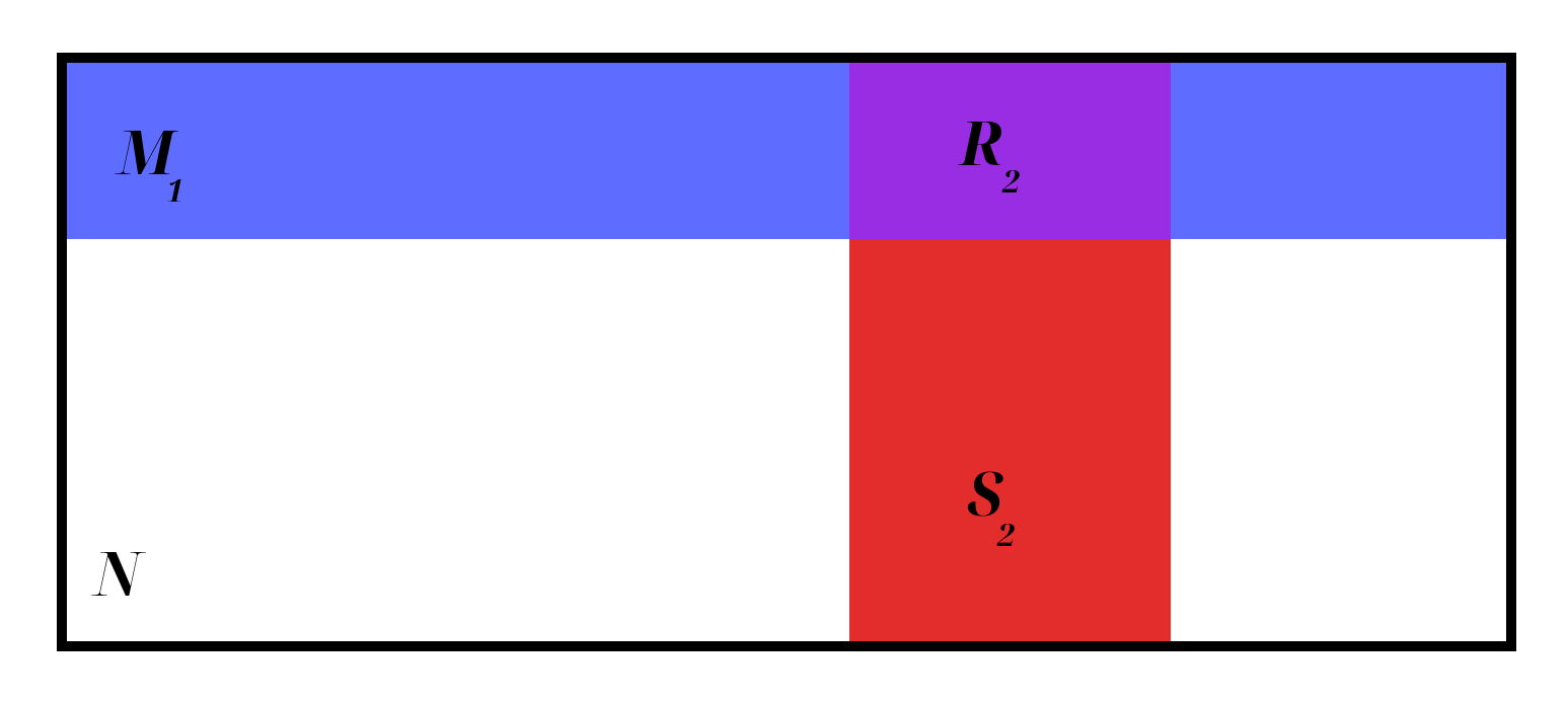
Some animals caught on the second sampling period (total number caught in second sample \(= S_2\)) will be re-captures of those marked on period one; the number of recaptures is represented by \(R_2\).
\(\frac{R_2}{S_2} = \frac{M_1}{N}\).

Thus, we can estimate the population size as: \[\hat{N} = \frac{S_2 M_1}{R_2}\]

In other words, \(R_2/M_1\) estimates the fraction of \(N\) marked on the first day. This can be shown graphically as follows (\(N\) is the entire box, \(M_1\) is the blue row, \(S_2\) is the red column, and \(R_2\) is their purple intersection):

MRR Diagram

Assumptions of the Lincoln-Petersen method:

Marks do not affect animals.
Marked animals are mixed in the population.
Marked and unmarked animals have the same probability of capture
The population is closed (no birth/death/migration)
Marks are not lost between samples

Although we can never be sure that the estimated population size \((\hat{N})\) equals the true value, \(\hat{N}\) should approach \(N\) as \(M_1\) and \(S_2\) get larger. Even though intense enough sampling could allow direct measure of \(N\), real habitats are too complex and mobile animals too elusive. In this exercise, we will study a hybrid population of Heliconius butterflies.

11.1.2 Heliconius butterflies

Our main focus for this exercise will be an enclosed hybrid population of Heliconius melopomene x Heliconius cydno. The exercise sits at the interface of population ecology and genetics since the study population is polymorphic for wing patterns reflecting a naturally occurring phenomenon in South America. It is known that males of Heliconius melpomene mate with females of Heliconius cydno in nature to yield species called H. heurippa, H. timareta, and likely others. Heliconius timareta displays a variety of color pattern types in different parts of its range. Such races are locally monomorphic (i.e. only one pattern exists in a particular place) However, genomic studies confirm that these populations share cydno mitochondrial haplotypes and a common mode of origination, in spite of diverse phenotypes. In the 1980s, Dr. Gilbert carried out studies of hybridization in H. cydno and H. melpomene in UT greenhouses and hypothesized the likely hybrid origin of species like H. timerata. Now that genomic studies verify his hypotheses on the origin of such species, Dr. Gilbert has recreated a hybrid population according to the likely mode of origin of H. timareta. This population is large and diverse in color pattern phenotypes for which we know the genetics of major pattern elements.

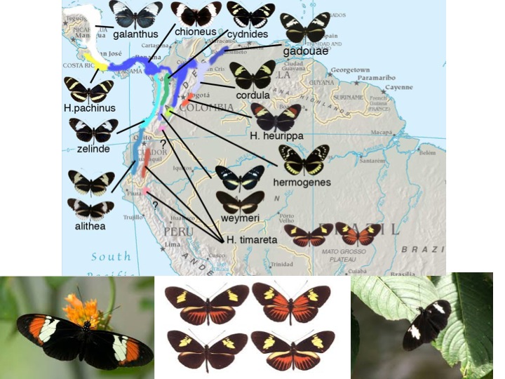
Distribution of some Heliconius species

With the hybrid H. cydno X H. melpomene population, you will be able to combine ecology and population genetics by applying Hardy-Weinberg law to test whether a force like selection or non-random mating is acting on wing pattern genes. Larry will photograph each numbered butterfly and post in a web album so that you can record the proportion of phenotypes and determine whether they are in Hardy-Weinberg equilibrium.

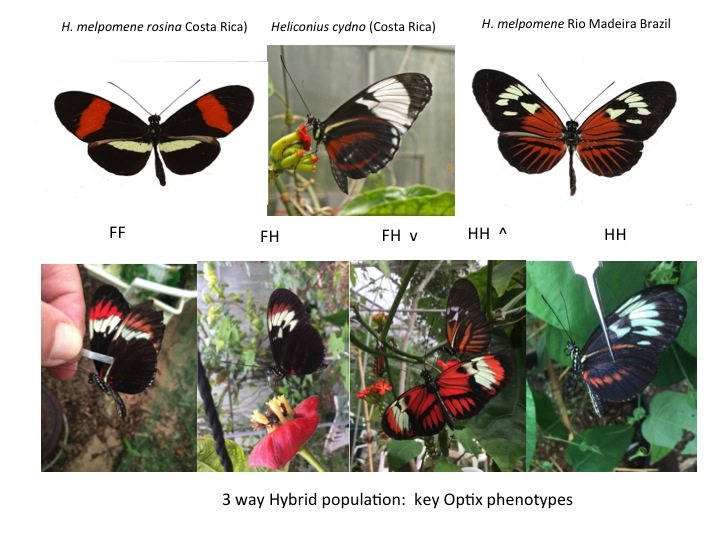
Optix phenotypes

We will score the orange/red/brown patterns for which the link between phenotype and genotype is now known. The mimetic phenotypes generated are key to the diversification of the genus, to predator protection niches, and to mutualism between sympatric species (Mullerian mimicry). A supergene locus controls expression of a transcription factor called Optix; this locus exhibits incomplete dominance, so the genotype can be directly determined from the phenotype. One allele (F) accounts for the red, orange, red or brown scales in the distal forewing band (beyond the large wing cell). Another allele (H) controls the presence of such scales on the hind wing and/or on the proximal FW in the cell region. We will use these genotypes to estimate whether the population is in Hardy-Weinberg Equilibirum

11.1.3 Hardy-Weinberg Equilibrium

A few definitions are in order:

Allele: one variant of a gene. For example, the Optix gene has the alleles \(F\) and \(H\).
Genotype: in a diploid organism like Heliconius butterflies, there are two copies of most genes; the genotype is the combination of the alleles. For Optix, genotypes can be \(FF\), \(FH\), or \(HH\). An individual with 2 of the same alleles (\(FF\) or \(HH\)) is a homozygote, while an individual with different alleles (\(FH\)) is a heterozygote.
Allele frequency: the proportion of each allele of a gene within a population. For 2-allele systems, we usually note these frequencies as \(p\) and \(q\), where \(p + q = 1\). In Optix, \(p\) is the frequency of \(F\) and \(q\) is the frequency of \(H\).
Genotype frequency: the proportion of each genotype within a population. For Optix, we will be noting these as \(f_{FF}\), \(f_{FH}\), and \(f_{HH}\). Genotype frequencies will also sum to 1.

Allele frequencies can be directly calculated from genotype frequencies \((p=f_{FF}+0.5*f_{FH}\), \(q=1-p)\). However, the reverse is not necessarily true. There are many possible genotype frequencies that can correspond to the same allele frequencies; as an extreme example, a population with 100 heterozygotes (\(FH\) genotypes) would have the same allele frequencies as one with 50 \(FF\) and \(50\) HH homozygotes. However, the two populations would look quite different. The relation between allele and genotype frequencies can help us understand a population’s biology.

11.1.3.1 Genotype frequencies at equilibrium

If genotype frequencies are stable and unchanging from one generation to the next, then we can expect a certain relationship between genotype and allele frequencies:

\[f_{FF}=p^{2};\,\,\,\,\,\,\,f_{FH}=2pq;\,\,\,\,\,\,\,f_{HH}=q^{2}\] This is called Hardy-Weinberg Equilibrium (HWE). An easy way to remember this is that genotypes take two alleles, so expanding the equation \((p+q)^{2}=1\) will give you these ratios. HWE only applies for a population that is not changing.

What can affect allele or genotype frequencies?

Natural selection: If one allele or genotype provides an advantage in the current environment, individuals with this allele are likely to produce more offspring, which will increase the allele frequency over time.
Migration: Allele frequencies tend to vary between populations of the same species; individuals moving from one population to another will make the allele frequencies more similar to each other.
Genetic drift: Variation in individual mating success will cause random changes in allele frequencies, in large populations, these are so small that they usually average out; however, small populations can have substantial change between generations.
Mutation: Random events can introduce new alleles; while this is rare and most mutations disappear through drift shortly after popping up, mutation is ultimately the source of all genetic variation.
Non-random mating: If individuals prefer to mate with like individuals, this can increase the frequencies of homozygous genotypes; conversely, a preference for different individuals can increase heterozygote frequencies. Unlike the previous four, non-random mating changes genotype frequencies without changing allele frequencies.

Pretty much any natural population will violate at least one of these conditions. So why is HWE useful? It gives us a baseline expectation to compare our observed genotype frequencies to. If our data are significantly different from the HWE values, we can conclude that one of these processes is playing an important role in the population. If not, then these processes are minor enough that we can ignore them.

11.1.3.2 Detecting violations of HWE

To test whether our genotype data is in Hardy-Weinberg equilibrium, we can use a chi-squared test of goodness-of-fit. First, we’ll need to calculate a chi-squared test statistic, which measures how strongly our observed data \((O)\) deviates from the HWE expectations \((E)\).

\[\chi^{2}=\sum_{i}\frac{\left(O_{i}-E_{i}\right)^{2}}{E_{i}}\]

In terms of our data, this is equal to

\[\chi^{2}=\frac{\left(f_{FF}-p^{2}\right)^{2}}{p^{2}}+\frac{\left(f_{FH}-2pq\right)^{2}}{2pq}+\frac{\left(f_{HH}-q^{2}\right)^{2}}{q^{2}}\]

This is somewhat different from the chi-squared tests we’ve done in previous labs (which are chi-squared tests of independence).

11.2 Questions and hypotheses

Primary Questions:

How does sampling intensity improve mark-release-recapture (MRR) population size estimates?
Does separating animals by sex alter our estimate of population size? What’s the sex ratio?
How does the Lincoln-Petersen model compare with alternate MRR methods?
Are the Heliconius populations in Hardy-Weinberg equilibrium for the Optix gene?

11.3 Field Methods

For the MRR exercise, your team will enter the greenhouse capture butterflies for two distinct periods.

For the first period, your group will capture 5 different butterflies. re-mixes with the population. At least thirty minutes after you’ve completed the first period, return to the greenhouse for the second period and capture five more. The delay should give the butterflies time to mix with the population.

Space yourselves out and move slowly around your area of the greenhouse when searching.
For each butterfly, record its number (or bring it to Dr. Gilbert if it doesn’t have one).
Butterflies often land and sit after capture; don’t resample these. Instead, scare them into flight (by gently waving your hand) to insure mixing of individuals in the population.

After you’ve completed your data collection, you will be given a photo album of the marked butterflies; you will need to identify the genotype and sex of the butterflies in the images for the Hardy-Weinberg exercise.

11.4 Analysis

The Lincoln-Petersen model:

If \(S_2\) is the number of individuals collected in a sample period, \(M_1\) is total number of previously marked individuals, and \(R_2\) is the number of marked individuals who were recaptured, then you can estimate population size:

\[\hat{N} = \frac{S_2 M_1}{R_2}\]

11.4.1 Effect of sampling intensity on Lincoln-Petersen \(\hat{N}\) estimates

We’re going to simulate increased sampling estimates by pooling together estimates from each team. I’ll be combining the data from each group in all possible team combinations (i.e., one team: A, B, C, …; two teams: AB, AC, AD, …; three teams: ABC, ABD, BCD, …). For each combination, you’ll need to calculate the Lincoln-Petersen population size estimate \((\hat{N})\). Create a figure showing the effect of sample size on \(\hat{N}\).

11.4.2 Sex ratios

Using the combined data from all teams, estimate \(\hat{N}\) separately for male and female butterflies. How does the sum of these estimates compare with the estimate when the sexes are lumped together?

What is the sex ratio of the population? Does it differ from 50:50? Use a chi-square test to test this.

11.4.3 Comparison of Lincoln-Petersen with alternative method

In 1970-71, Larry Gilbert collected data on a natural population of Heliconius in Trinidad (recall his paper spreadsheet from lecture with cells colored in to represent individuals). We will use this method to estimate population sizes.

For each of the three sample periods, use a regression to model the relationship between the daily recapture proportion \((x)\) and the cumulative number of individuals marked \((y)\). Intuitively, a recapture rate of 1.0 would suggest that you’ve sampled the entire population; you could thus use this regression equation to estimate \((\hat{N})\) by evaluating it when \(x=1\). Create a multi-panel regression plot to go along with these methods.

Compare these estimates with the Lincoln-Petersen estimate from the day with the highest proportion of recaptures in the sampling period.

11.4.4 Hardy-Weinberg

First, you’ll want to get the observed numbers for each genotype; we’ll call these \(N_{FF}\), \(N_{FH}\), and \(N_{HH}\); the total sample size \(N\) is the sum of these.

From these observed genotypes, you can calculate the genotype frequency of F, which is just \(\frac{N_{FF} + 0.5 N_{FH} }{N}\)l let’s call this \(p\).

You can get your HWE expected genotypes by using \(p\) and \(q=1-p\) to get your expected genotype frequencies; From here, you can run a chi-squared test.

11.5 Discussion

You should address the following in your discussion:

How well did we meet the assumptions of MRR?
Our MRR data came from a closed population; briefly speculate about some of the potential problems with these estimates in an open, natural population (how would emigration/immigration or birth/death affect the estimates)? How might our study compare with data from a natural population?
How well does the Lincoln-Petersen model compare with fractional recapture estimation in a natural population? How different were your population estimates? What factors could help explain them?
Think of some creative ways you could improve sampling in an MRR project (beyond just increasing the sample size).
Don’t forget to discuss your results from the sex ratio and genotype analyses.